Introduction to Digital Imaging in Microscopy

Part II: Basic Microscopy Concepts

Multidimensional Imaging

The term multidimensional imaging can be used to describe three-dimensional imaging (3D; volume), four-dimensional imaging (4D; volume and time) or imaging in 5 or more dimensions (5D, 6D, etc., volume, time, wavelength), each representing a combination of different variables. Modern bioscience applications increasingly require optical instruments and digital image processing systems capable of capturing quantitative, multidimensional information about dynamic, spatially complex specimens. Multidimensional, quantitative image analysis has become essential to a wide assortment of bioscience applications. The imaging of sub-resolution objects, rapid kinetics and dynamic biological processes present technical challenges for instrument manufacturers to produce ultra sensitive, extremely fast and accurate image acquisition and processing devices.

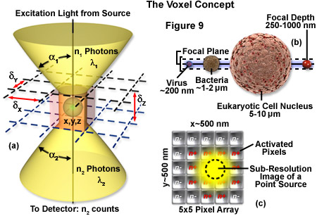
The image produced by the microscope and projected onto the surface of the detector is a two dimensional representation of an object that exists in three dimensional space. As discussed in Part I, the image is divided into a two dimensional array of pixels, represented graphically by an x and y axis. Each pixel is a typically square area determined by the lateral resolution and magnification of the microscope as well as the physical size of the detector array. Similar to the pixel in 2D imaging, a volume element or voxel, having dimensions defined by x, y and z axes, is the basic unit or sampling volume in 3D imaging. A voxel represents an optical section, imaged by the microscope, that is comprised of the area resolved in the x-y plane and a distance along the z axis defined by the depth of field, as illustrated in Figure 9. To illustrate the voxel concept (Figure 9), a sub-resolution fluorescent point object can be described in three dimensions with a coordinate system, as illustrated in Figure 9(a). The typical focal depth of an optical microscope is shown relative to the dimensions of a virus, bacteria, and mammalian cell nucleus in Figure 9(b), whereas Figure 9(c) depicts a schematic drawing of a sub-resolution point image projected onto a 25-pixel array. Activated pixels (those receiving photons) span a much larger dimension than the original point source.

The depth of field is a measurement of object space parallel with the optical axis. It describes the numerical aperture-dependent, axial resolution capability of the microscope objective and is defined as the distance between the nearest and farthest objects in simultaneous focus. Numerical aperture (NA) of a microscope objective is determined by multiplying the sine of one-half of the angular aperture by the refractive index of the imaging medium. Lateral resolution varies inversely with the first power of the NA, whereas axial resolution is inversely related to the square of the NA. The NA therefore affects axial resolution much more so than lateral resolution. While spatial resolution depends only on NA, voxel geometry depends on the spatial resolution as determined by the NA and magnification of the objective, as well as the physical size of the detector array. With the exception of multiphoton imaging, which uses femtoliter voxel volumes, widefield and confocal microscopy are limited to dimensions of about 0.2 micrometers x 0.2 micrometers x 0.4 micrometers based on the highest NA objectives available.

Virus sized objects that are smaller than the optical resolution limits, can be detected but are poorly resolved. In thicker specimens, such as cells and tissues, it is possible to repeatedly sample at successively deeper layers so that each optical section contributes to a z series (or z stack). Microscopes that are equipped with computer controlled step motors acquire an image then adjust the fine focus according to the sampling parameters, take another image, and continue until a large enough number of optical sections have been collected. The step size is adjustable and will depend, as for 2D imaging, on appropriate Nyquist sampling. The axial resolution limit is larger than the limit for lateral resolution. This means that the voxel may not be an equal-sided cube and will have a z dimension that can be several times greater than the x and y dimensions. For example, a specimen can be divided into 5-micrometers thick optical sections and sampled at 20-micrometer intervals. If the x and y dimensions are 0.5 micrometers x 0.5 micrometers then the resulting voxel will be 40 times longer than it is wide.

Three dimensional imaging can be performed with conventional widefield fluorescence microscopes equipped with a mechanism to acquire sequential optical sections. Objects in a focal plane are exposed to an illumination source and light emitted from the fluorophore is collected by the detector. The process is repeated at fine focus intervals along the z axis, often hundreds of times, and a sequence of optical sections or z series (also z stack) is generated. In widefield imaging of thick biological samples blurred light and scatter can degrade the quality of the image in all three dimensions.

Confocal microscopy has several advantages that have made it a commonly used instrument in multidimensional, fluorescence microscopy. In addition to slightly better lateral and axial resolution, a laser scanning confocal microscope (LSCM) has a controllable depth of field, eliminates unwanted wavelengths and out of focus light, and is able to finely sample thick specimens. A system of computer controlled, galvanometer driven dichroic mirrors direct an image of the pinhole aperture across the field of view, in a raster pattern similar to that used in television. An exit pinhole is placed in a conjugate plane to the point on the object being scanned. Only light emitted from the point object is transmitted through the pinhole and reaches the detector element. Optical section thickness can be controlled by adjusting the diameter of the pinhole in front of the detector, a feature that enhances flexibility in imaging biological specimens. Technological improvements such as computer and electronically controlled laser scanning and shuttering, as well as variations in the design of instruments (such as spinning disk, multiple pinhole and slit scanning versions) have increased image acquisition speeds. Faster acquisition and better control of the laser by shuttering the beam reduces the total exposure effects on light sensitive, fixed or live cells. This enables the use of intense, narrow wavelength bands of laser light to penetrate deeper into thick specimens making confocal microscopy suitable for many time resolved, multidimensional imaging applications.

For multidimensional applications in which the specimen is very sensitive to visible wavelengths, the sample volume or fluorophore concentration is extremely small, or when imaging through thick tissue specimens, laser scanning multiphoton microscopy (LSMM; often simply referred to as multiphoton microscopy) is sometimes employed. While the scanning operation is similar to that of a confocal instrument, LSMM uses an infrared illumination source to excite a precise femtoliter sample volume (approximately 10E-15 liters). Photons are generated by an infrared laser and localized in a process known as photon crowding. The simultaneous absorption of two low energy photons is sufficient to excite the fluorophore and cause it to emit at its characteristic, stokes shifted wavelength. The longer wavelength excitation light causes less photobleaching and phototoxicity and, as a result of reduced Rayleigh scattering, penetrates further into biological specimens. Due to the small voxel size, light is emitted from only one diffraction limited point at a time, enabling very fine and precise optical sectioning. Since there is no excitation of fluorophores above or below the focal plane, multiphoton imaging is less affected by interference and signal degradation. The absence of a pinhole aperture means that more of the emitted photons are detected which, in the photon starved applications typical of multidimensional imaging, may offset the higher cost of multiphoton imaging systems.

The z series is often used to represent the optical sections of a time lapse sequence where the z axis represents time. This technique is frequently used in developmental biology to visualize physiological changes during embryo development. Live cell or dynamic process imaging often produces 4D data sets. These time resolved volumetric data are visualized using 4D viewing programs and can be reconstructed, processed and displayed as a moving image or montage. Five or more dimensions can be imaged by acquiring the 3- or 4-dimensional sets at different wavelengths using different fluorophores. The multi-wavelength optical sections can later be combined into a single image of discrete structures in the specimen that have been labeled with different fluorophores. Multidimensional imaging has the added advantage of being able to view the image in the x-z plane as a profile or vertical slice.

The Point Spread Function

The ideal point spread function (PSF) is the three-dimensional diffraction pattern of light emitted from an infinitely small point source in the specimen and transmitted to the image plane through a high NA objective. It is considered to be the fundamental unit of an image in theoretical models of image formation. When light is emitted from such a point object, a fraction of it is collected by the objective and focused at a corresponding point in the image plane. However, the objective lens does not focus the emitted light to an infinitely small point in the image plane. Rather, light waves converge and interfere at the focal point to produce a diffraction pattern of concentric rings of light surrounding a central, bright disk, when viewed in the x-y plane. The radius of disk is determined by the NA, thus the resolving power of an objective lens can be evaluated by measuring the size of the Airy disk. The image of the diffraction pattern can be represented as an intensity distribution as shown in Figure 10. The bright central portion of the Airy disk and concentric rings of light correspond to intensity peaks in the distribution. In Figure 10, relative intensity is plotted as a function of spatial position for PSFs from objectives having numerical apertures of 0.3 and 1.3. The full-width at half maximum (FWHM) is indicated for the lower NA objective along with the Rayleigh limit.

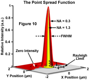
In a perfect lens with no spherical aberration the diffraction pattern at the paraxial (perfect) focal point is both symmetrical and periodic in the lateral and axial planes. When viewed in either axial meridian (x-z or y-z) the diffraction image can have various shapes depending on the type of instrument used (i.e. widefield, confocal or multiphoton) but is often hourglass or football-shaped. The point spread function is generated from the z series of optical sections and can be used to evaluate the axial resolution. As with lateral resolution, the minimum distance the diffraction images of two points can approach each other and still be resolved is the axial resolution limit. The image data are represented as an axial intensity distribution in which the minimum resolvable distance is defined as the first minimum of the distribution curve.

The PSF is often measured using a fluorescent bead embedded in a gel that approximates an infinitely small point object in a homogeneous medium. However, thick biological specimens are far from homogeneous. Differing refractive indices of cell materials, tissues or structures in and around the focal plane can diffract light and result in a PSF that deviates from design specification, fluorescent bead determination or the calculated, theoretical PSF. A number of approaches to this problem have been suggested including comparison of theoretical and empirical PSFs, embedding a fluorescent microsphere in the specimen or measuring the PSF using a subresolution object native to the specimen.

The PSF is valuable not only for determining the resolution performance of different objectives and imaging systems, but also as a fundamental concept used in deconvolution. Deconvolution is a mathematical transformation of image data that reduces out of focus light or blur. Blurring is a significant source of image degradation in 3D widefield fluorescence microscopy. It is nonrandom and arises within the optical train and specimen, largely as a result of diffraction. A computational model of the blurring process, based on the convolution of a point object and its PSF, can be used to deconvolve or reassign out of focus light back to its point of origin. Deconvolution is used most often in 3D widefield imaging. However, images produced with confocal, spinning disk and multiphoton microscopes can also be improved using image restoration algorithms.

Image formation begins with the assumptions that the process is linear and shift invariant. If the sum of the images of two discrete objects is identical to the image of the combined object the condition of linearity is met, providing the detector is linear and quenching and self-absorption by fluorophores is minimized. When the process is shift invariant, the image of a point object will be the same everywhere in the field of view. Shift invariance is an ideal condition that no real imaging system meets. Nevertheless, the assumption is reasonable for high quality research instruments.

Convolution mathematically describes the relationship between the specimen and its optical image. Each point object in the specimen is represented by a blurred image of the object (the PSF) in the image plane. An image consists of the sum of each PSF multiplied by a function representing the intensity of light emanating from its corresponding point object:

i(x) = o(x - x') × psf(x')dx'

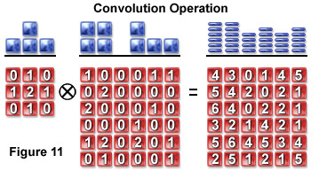
A pixel blurring kernel is used in convolution operations to enhance the contrast of edges and boundaries and the higher spatial frequencies in an image. Figure 11 illustrates the convolution operation using a 3 x 3 kernel to convolve a 6 x 6 pixel object. Above the arrays in Figure 11 are profiles demonstrating the maximum projection of the two-dimensional grids when viewed from above.

An image is a convolution of the object and the PSF and can be symbolically represented as follows:

image(r) = object(r) ⊗ psf(r)

where the image, object and PSF are denoted as functions of position (r) or an x, y, z and t (time) coordinate. The Fourier transform shows the frequency and amplitude relationship between the object and point spread function, converting the space variant function to a frequency variant function. Because convolution in the spatial domain is equal to multiplication in the frequency domain, convolutions are more easily manipulated by taking their Fourier transform (F).

F{i(x,y,z,t)} = F{o(x,y,z,t)} × F{psf(x,y,z,t)}

In the spatial domain described by the PSF, a specimen is a collection of point objects and the image is a superposition or sum of point source images. The frequency domain is characterized by the optical transfer function (OTF). The OTF is the Fourier transform of the PSF and describes how spatial frequency is affected by blurring. In the frequency domain the specimen is equivalent to the superposition of sine and cosine functions and the image consists of the sum of weighted sine and cosine functions. The Fourier transform further simplifies the representation of the convolved object and image such that the transform of the image is equal to the specimen multiplied by the OTF. The microscope passes low frequency (large, smooth) components best, intermediate frequencies are attenuated and high frequencies greater than 2NA/λ are excluded. Deconvolution algorithms are therefore required to augment high spatial frequency components.

Theoretically, it should be possible to reverse the convolution of object and PSF by taking the inverse of the Fourier transformed functions. However, deconvolution increases noise which exists at all frequencies in the image. Beyond half the Nyquist sampling frequency no useful data are retained but noise is nevertheless amplified by deconvolution. Contemporary image restoration algorithms use additional assumptions about the object such as smoothness or non-negative value and incorporate information about the noise process to avoid some of the noise related limitations.

Deconvolution algorithms are of two basic types. Deblurring algorithms use the PSF to estimate blur then subtract it by applying the computational operation to each optical section in a z-series. Algorithms of this type include nearest neighbor, multi neighbor, no neighbor and unsharp masking. The more commonly used nearest neighbor algorithm estimates and subtracts blur from z sections above and below the section to be sharpened. While these run quickly and use less computer memory, they don't account for cross-talk between distant optical sections. Deblurring algorithms may decrease the SNR by adding noise from multiple planes. Images of objects whose PSFs overlap in the paraxial plane can often be sharpened by deconvolution, however, at the cost of displacement of the PSF. Deblurring algorithms introduce artifacts or changes in the relative intensities of pixels and thus can't be used for morphometric measurements, quantitative intensity determinations or intensity ratio calculations.

Image restoration algorithms use a variety of methods to reassign out of focus light to its proper position in the image. These include inverse filter types such as Wiener deconvolution or linear least squares, constrained iterative methods such as Jansson van Cittert, statistical image restoration and blind deconvolution. Constrained deconvolution imposes limitations by excluding non-negative pixels and placing finite limits on size or fluorescent emission, for example. An estimation of the specimen is made and an image calculated and compared to the recorded image. If the estimation is correct, constraints are enforced and unwanted features are excluded. This process is convenient to iterative methods that repeat the constraint algorithm many times. The Jansson van Cittert algorithm predicts an image, applies constraints and calculates a weighted error that is used to produce a new image estimate for multiple iterations. This algorithm has been effective in reducing high frequency noise.

Blind deconvolution does not use a calculated or measured PSF but rather, calculates the most probable combination of object and PSF for a given data set. This method is also iterative and has been successfully applied to confocal images. Actual PSFs are degraded by the varying refractive indices of heterogeneous specimens. In CLSM where light levels are typically low, this effect is compounded. Blind deconvolution reconstructs both the PSF and the deconvolved image data. Compared with deblurring algorithms, image restoration methods are faster, frequently result in better image quality and are amenable to quantitative analysis.

Deconvolution performs its operations using floating point numbers and consequently, uses large amounts of computing power. Four bytes per pixel are required which translates to 64 Mb for a 512 x 512 x 64 image stack. Deconvolution is also CPU intensive and large data sets with numerous iterations may take several hours to produce a fully restored image depending on processor speed. Choosing an appropriate deconvolution algorithm involves determining a delicate balance of resolution, processing speed and noise that is correct for a particular application.

Digital Image Display and Storage

The display component of an imaging system reverses the digitizing process accomplished in the A/D converter. The array of numbers representing image signal intensities must be converted back into an analog signal (voltage) in order to be viewed on a computer monitor. A problem arises when the function (sin(x)/x) representing the waveform of the digital information must be made to fit the simpler Gaussian curve of the monitor scanning spot. To perform this operation without losing spatial information, the intensity values of each pixel must undergo interpolation, a type of mathematical curve fitting. The deficiencies related to the interpolation of signals can be partially compensated for by using a high resolution monitor that has a bandwidth greater than 20 megaHertz, as do most modern computer monitors. Increasing the number of pixels used to represent the image by sampling in excess of the Nyquist limit (oversampling) increases the pixel data available for image processing and display.

A number of different technologies are available for displaying digital images though microscopic imaging applications most often use monitors based on either cathode ray tube (CRT) or liquid crystal display (LCD) technology. These display technologies are distinguished by the type of signals each receives from a computer. LCD monitors accept digital signals which consist of rapid electrical pulses that are interpreted as a series of binary digits (0 or 1). CRT displays accept analog signals and thus require a digital to analog converter (DAC) that precedes the monitor in the imaging process train.

Digital images can be stored in a variety of file formats that have been developed to meet different requirements. The format used depends on the type of image and how it will be presented. Quality, high resolution images require large file sizes. File sizes can be reduced by a number of different compression algorithms but image data may be lost depending on the type. Lossless compressions (such as Tagged Image File Format; TIFF) encode information more efficiently by identifying patterns and replacing them with short codes. These algorithms can reduce an original image by about 50 to 75 percent. This type of file compression can facilitate transfer and sharing of images and allows decompression and restoration to the original image parameters. Lossy compression algorithms, such as that used to define pre-2000 JPEG image files, are capable of reducing images to less than 1 percent of their original size. The JPEG 2000 format uses both types of compression. The large reduction is accomplished by a type of undersampling in which imperceptible grey level steps are eliminated. Thus the choice is often a compromise between image quality and manageability.

Bit mapped or raster based images are produced by digital cameras, screen and print output devices that transfer pixel information serially. A 24 bit color (RGB) image uses 8 bits per color channel resulting in 256 values for each color for a total of 16.7 million colors. A high resolution array of 1280 x 1024 pixels representing a true color 24 bit image would require more than 3.8 megabytes of storage space. Commonly used raster based file types include GIF, TIFF, and JPEG. Vector based images are defined mathematically and used for primarily for storage of images created by drawing and animation software. Vector imaging typically requires less storage space and is amenable to transformation and resizing. Metafile formats, such as PDF, can incorporate files created by both raster and vector based images. This file format is useful when images must be consistently displayed in a variety of applications or transferred between different operating systems.

As the dimensional complexity of images increases image file sizes can become very large. For a single color, 2048 x 2048 image file size is typically about 8 megabytes. A multicolor image of the same resolution can reach 32 megabytes. For images with 3 spatial dimensions and multiple colors a smallish image might require 120 megabytes or more of storage. In live cell imaging where time resolved, multidimensional images are collected, image files can become extremely large. For example, an experiment that uses 10 stage positions, imaged over 24 hours with 3-5 colors at one frame per minute, a 1024 x 1024 frame size, and 12 bit image could amount to 86 gigabytes per day! High speed confocal imaging with special storage arrays can produce up to 100 gigabytes per hour. Image files of this size and complexity must be organized and indexed and often require massive directories with hundreds of thousand of images saved in a single folder as they are streamed from the digital camera. Modern hard drives are capable of storing at least 500 gigabytes. The number of images that can be stored depends on the size of the image file. About 250,000 2-3 megabyte images can be stored on most modern hard drives. External storage and backup can be performed using compact disks (CDs) that hold about 650 megabytes or DVDs that have 5.2 gigabyte capacities. Image analysis typically takes longer than collection and is presently limited by computer memory and drive speed. Storage, organization, indexing, analysis and presentation will be improved as 64 bit multiprocessors with large memory cores become available.

Imaging Modes in Optical Microscopy

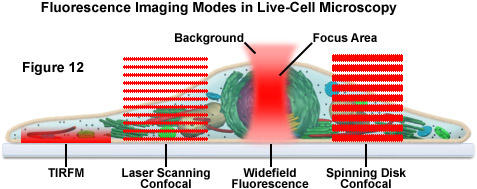
The imaging of living cells and organisms has traditionally been based on long term time lapse experiments designed to observe cell movement and dynamic events (see Figure 12). Techniques have typically included brightfield, polarized light microscopy, differential interference contrast (DIC), Hoffman modulation contrast (HMC), phase contrast, darkfield and widefield fluorescence. In the past decade, a number of new imaging technologies have been developed that have enabled time lapse imaging to be integrated with techniques that monitor, quantify and perturb dynamic processes in living cells and organisms. Laser scanning confocal, spinning disk confocal, laser scanning multiphoton and total internal reflection (TIRFM) microscopy have generated a wide variety of techniques that have facilitated greater insights into dynamic biological processes

Until recently, live cell imaging has involved adherent mammalian cells, positioned a short distance (approximately 10 micrometers or less) from the cover slip/medium interface. Specimens in a growing number of contemporary investigations are often 10-200 micrometers thick. There are a number of problems associated with imaging beyond a depth of 20-30 micrometers within a living specimen. Primary among the difficulties are blurring caused by out of focus light, movement within the cytoplasm that limits exposure time and, the photosensitivity of fluorophores and living cells that make them vulnerable to photobleaching and phototoxic effects. The imaging of living cells, tissues and organisms usually involves a compromise between image resolution and maintaining conditions requisite to the survival and normal biological functioning of the specimen

Traditional approaches to live-cell imaging are often based on short or long term time-lapse investigations designed to monitor cellular motility and dynamic events using common contrast enhancement techniques, including brightfield, DIC, HMC, phase contrast, and widefield fluorescence. However, modern techniques and newly introduced methodologies are extending these observations well beyond simply creating cinematic sequences of cell structure and function, thus enabling time-lapse imaging to be integrated with specialized modes for monitoring, measuring, and perturbing dynamic activities of tissues, cells, and subcellular structures.

A majority of the live-cell imaging investigations are conducted with adherent mammalian cells, which are positioned within 10 micrometers of the coverslip-medium interface. Increasingly, however, investigators are turning their attention to thicker animal and plant tissue specimens that can range in thickness from 10 to 200 micrometers. In this case, out of focus information blurs the image and the constant churning of the cytoplasm creates limitations on exposure times. Both brightfield and fluorescence methods used in imaging thicker animal tissues and plants must take into account the sensitivity of these specimens to light exposure and the problems associated with resolving features that reside more than 20 to 30 micrometers within the specimen.

Brightfield techniques are often less harmful to living cells, but methodology for observing specific proteins using trans-illumination have not been widely developed. Generating a high-contrast chromatic (color) or intensity difference in a brightfield image is more difficult than identifying a luminous intensity change (in effect, due to fluorescence) against a dark or black background. Therefore, brightfield techniques fine applications in following organelles or cell-wide behavior, while fluorescence methods, including confocal techniques, are generally used for following specific molecules.

Presented in Figure 12 is a schematic illustration of popular imaging modes in widefield and scanning modes of fluorescence microscopy. Widefield, laser scanning, spinning disk, and multiphoton techniques employ vastly different illumination and detection strategies to form an image. The diagram illustrates an adherent mammalian cell on a coverslip being illuminated with total internal reflection, laser scanning and spinning disk confocal, in addition to traditional widefield fluorescence. The excitation patterns for each technique are indicated in red overlays. In widefield, the specimen is illuminated throughout the field as well as above and below the focal plane. Each point source is spread into a shape resembling a double-inverted cone (the point-spread function). Only the central portion of this shape resides in the focal plane with the remainder contributing to out-of-focus blur, which degrades the image.

In contrast the laser scanning, multiphoton, and spinning disk confocal microscopes scan the specimen with a tightly focused laser or arc-discharge lamp (spinning disk). The pattern of excitation is a point-spread function, but a conjugate pinhole in the optical path of the confocal microscopes prevents fluorescence originating away from the focal plane from impacting the photomultiplier or digital camera detector. The laser scanning confocal microscope has a single pinhole and a single focused laser spot that is scanned across the specimen. In the spinning disk microscope, an array of pinhole or slit apertures, in some cases fitted with microlenses, is placed on a spinning disk such that the apertures rapidly sweep over the specimen and create an image recorded with an area array detector (digital camera). In the multiphoton microscope, the region at which photon flux is high enough to excite fluorophores with more than one photon resides at the in-focus position of the point-spread function. Thus, fluorophore excitation only occurs in the focal plane. Because all fluorescence emanates from in-focus fluorophores, no pinhole is required and the emitted fluorescence generates a sharp, in-focus image.

One of the primary and favorite techniques used in all forms of optical microscopy for the past three centuries, brightfield illumination relies upon changes in light absorption, refractive index, or color for generating contrast. As light passes through the specimen, regions that alter the direction, speed, and/or spectrum of the wavefronts generate optical disparities (contrast) when the rays are gathered and focused by the objective. Resolution in a brightfield system depends on both the objective and condenser numerical apertures, and an immersion medium is often required on both sides of the specimen (for numerical aperture combinations exceeding a value of 1.0). Digital cameras provide the wide dynamic range and spatial resolution required to capture the information present in a brightfield image. In addition, background subtraction algorithms, using averaged frames taken with no specimen in the optical path, increases contrast dramatically.

Simple brightfield imaging, with the microscope properly adjusted for Köhler illumination, provides a limited degree of information about the cell outline, nuclear position, and the location of larger vesicles in unstained specimens. Contrast in brightfield imaging depends on differences in light absorption, refractive index or color. Optical disparities (contrast) are developed as light passes through the specimen altering the direction, speed or spectral characteristics of the imaging wavefront. The technique is more useful with specimens stained with visible light absorbing dyes (such as eosin and hematoxylin; see Figure 13a). However, the general lack of contrast in brightfield mode when examining unstained specimens renders this technique relatively useless for serious investigations of living cell structure. Methods that enhance contrast include differential interference contrast, polarized light, phase contrast, Hoffman modulation contrast, and darkfield microscopy (examples are illustrated in Figure 13). Several of these techniques are limited by light originating in regions removed from the focal plane when imaging thicker plant and animal tissues, while polarized light requires birefringence (usually not present to a significant degree in animal cells) to generate contrast.

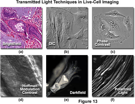
Figure 13 illustrates contrast-enhancing imaging modes in brightfield microscopy. In Figure 13(a), a thin section of human basal cell carcinoma stained with eosin and hematoxylin reveals intricate details of the affected tissue. Indian muntjac cells are imaged with DIC optics in Figure 13(b), whereas a similar culture of human cervical carcinoma (HeLa) cells are presented under phase contrast illumination in Figure 13(c). Mouse heart tissue bathed in saline is readily imaged in thin optical sections using HMC (Figure 13(d)), and similarly structured rabbit skeletal muscle is presented with polarized light in Figure 13(f). Darkfield microscopy (Figure 13(e)) is useful for a variety of imaging scenarios, in this case, to visualize a living Obelia hydroid in culture.

Differential interference contrast microscopy (Figure 13(b)) requires plane-polarized light and additional light-shearing (Nomarski) prisms to exaggerate minute differences in specimen thickness gradients and refractive index. Lipid bilayers, for example, produce excellent contrast in DIC because of the difference in refractive index between aqueous and lipid phases of the cell. In addition, cell boundaries in relatively flat adherent mammalian and plant cells, including the plasma membrane, nucleus, vacuoles, mitochondria, and stress fibers, which usually generate significant gradients, are readily imaged with DIC. In plant tissues, the birefringent cell wall reduces contrast in DIC to a limited degree, but a properly aligned system should permit visualization of nuclear and vacuolar membranes, some mitochondria, chloroplasts, and condensed chromosomes in epidermal cells. Differential interference contrast is an important technique for imaging thick plant and animal tissues because, in addition to the increased contrast, DIC exhibits decreased depth of focus at wide apertures, creating a thin optical section of the thick specimen. This effect is also advantageous for imaging adherent cells to minimize blur arising from floating debris in the culture medium.

Polarized light microscopy (Figure 13(f)) is conducted by viewing the specimen between crossed polarizing elements. Assemblies within the cell having birefringent properties, such as the plant cell wall, starch granules, and the mitotic spindle, as well as muscle tissue, rotate the plane of light polarization, appearing bright on a dark background. The rabbit muscle tissue illustrated in Figure 13(f) is an example of polarized light microscopy applied to living tissue observation. Note that this technique is limited by the rare occurrence of birefringence in living cells and tissues, and has yet to be fully explored. As mentioned above, differential interference contrast operates by placing a matched pair of opposing Nomarski prisms between crossed polarizers, so that any microscope equipped for DIC observation can also be employed to examine specimens in plane-polarized light simply by removing the prisms from the optical pathway.

The widely popular phase contrast technique (as illustrated in Figure 13(c)) employs an optical mechanism to translate minute variations in phase into corresponding changes in amplitude, which can be visualized as differences in image contrast. The microscope must be equipped with a specialized condenser containing a series of annuli matched to a set of objectives containing phase rings in the rear focal plane (phase contrast objectives can also be used with fluorescence, but with a slight reduction in transmission). Phase contrast is an excellent method to increase contrast when viewing or imaging living cells in culture, but typically results in excessive halos surrounding the outlines of edge features. These halos are optical artifacts that often reduce the visibility of boundary details. The technique is not useful for thick specimens (such as plant and animal tissue sections) because shifts in phase occur in regions removed from the focal plane that distort image detail. Furthermore, floating debris and other out-of-focus phase objects interfere with imaging adherent cells on coverslips.

Often metaphorically referred to as "poor man's DIC", Hoffman modulation contrast is an oblique illumination technique that enhances contrast in living cells and tissues by detection of optical phase gradients (see Figure 13(d)). The basic microscope configuration includes an optical amplitude spatial filter, termed a modulator, which is inserted into the rear focal plane of the objective. Light intensity passing through the modulator varies above and below an average value, which by definition, is then said to be modulated. Coupled to the objective modulator is an off-axis slit aperture that is placed in the condenser front focal plane to direct oblique illumination towards the specimen. Unlike the phase plate in phase contrast microscopy, the Hoffman modulator is designed not to alter the phase of light passing through; rather it influences the principal zeroth order maxima to produce contrast. Hoffman modulation contrast is not hampered by the use of birefringent materials (such as plastic Petri dishes) in the optical pathway, so the technique is more useful for examining specimens in containers constructed with polymeric materials. On the downside, HMC produces a number of optical artifacts that render the technique somewhat less useful than phase contrast or DIC for live-cell imaging on glass coverslips.

The methodology surrounding darkfield microscopy, although widely used for imaging transparent specimens throughout the nineteenth and twentieth centuries, is limited in use to physically isolated cells and organisms (as presented in Figure 13(e)). In this technique, the condenser directs a cone of light onto the specimen at high azimuths so that first-order wavefronts do not directly enter the objective front lens element. Light passing through the specimen is diffracted, reflected, and/or refracted by optical discontinuities (such as the cell membrane, nucleus, and internal organelles) enabling these faint rays to enter the objective. The specimen can then be visualized as a bright object on an otherwise black background. Unfortunately, light scattered by objects removed from the focal plane also contribute to the image, thus reducing contrast and obscuring specimen detail. This artifact is compounded by the fact that dust and debris in the imaging chamber also contribute significantly to the resulting image. Furthermore, thin adherent cells often suffer from very faint signal, whereas thick plant and animal tissues redirect too much light into the objective path, reducing the effectiveness of the technique.

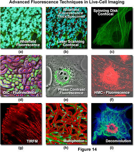
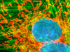
Widefield and point or slit scanning fluorescence imaging modes use divergent strategies to excite samples and detect the fluorescent signals as reviewed in Figure 14. The figure illustrates the different excitation patterns used in TIRFM, LSCM, multiphoton, and widefield fluorescence microscopy. In widefield fluorescence microscopy the sample is illuminated throughout the entire field, including the regions above and below the focal plane. The PSF in widefield fluorescence microscopy resembles a double inverted cone with its central portion in the focal plane. Light originating in areas adjacent to the focal plane contributes to blurring and image degradation (Figure 14(a); widefield fluorescence, rat brain hippocampus). While deconvolution can be used to reduce blur (Figure 14(i); mitosis in an epithelial cell), computational methods work better on fixed specimens than on live cell cultures due to the requirement for larger signal (longer exposure) and a homogeneous sample medium.

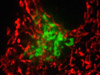
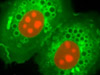
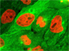
The advent of confocal (Figure 14(b); rat brain hippocampus), spinning disk (Figure 14(c); microtubules) and multiphoton (Figure 14(h); rabbit skeletal muscle with immunofluorescence) microscopy enabled thin and precise optical sectioning to greater depths within living samples. These imaging modes use a precisely focused laser or arc lamp (spinning disk) to scan the specimen in a raster pattern, and are often combined with conventional transmitted brightfield techniques, such as DIC, HMC, and phase contrast (see Figures 14(d; mouse kidney tissue with immunofluorescence), 14(e; Golgi apparatus in epithelial cell), and 14(f; mitochondria in a fibroblast cell)). The LSCM uses a single pinhole to produce an illumination spot that is scanned across the specimen. The use of conjugate pinholes in LSCM prevents out of focus light from reaching the detector. Spinning disk microscopy uses an array of pinhole or slit apertures and is able to scan rapidly across a specimen though it produces thicker optical sections than the single, stationary pinhole used in LSCM. Spinning disk modes are less effective at excluding out of focus information than LSCM but scan more rapidly without compromising photon throughput. Both confocal and spinning disk modes reduce blur and improve axial resolution. Confocal fluorescence microscopy is frequently limited by the low number of photons collected in the brightest pixels in the image. Multiphoton microscopy uses two or more lower energy photons (infrared) to excite a femtoliter sample volume, exciting only the fluorophores at the in focus position of the PSF. Multiphoton imaging therefore doesn't require pinholes to exclude out of focus light and collects a greater portion of the emitted fluorescence.

An emerging technique known as total internal reflection fluorescence microscopy (TIRFM; discussed above and see Figure 14(g); alpha-actinin cytoskeletal network near the coverslip) employs a laser source that enters the coverslip at a shallow angle and reflects off the surface of the glass without entering the specimen. Differences in refractive index (n1/n2) between the glass and the interior of a cell determine how light is refracted or reflected at the interface as a function of the incident angle. At the critical angle,

θ_critical = sin^-1(n₁/n₂)

a majority of the incident light is completely (totally) reflected from the glass/medium interface. The reflection within the coverslip leads to an evanescent surface wave (electromagnetic field) that has a frequency equal to the incident energy and is able to excite flurophores within 50-100 nanometers of the coverslip surface. TIRF works well for single molecule determinations and adherent mammalian cells because of the extreme limitation on the depth of excitation. Thick specimens are not well imaged because of the limited band of excitation. TIRF microscopy has wide application in imaging surface and interface fluorescence. For example, TIRF can be used to visualize cell/substrate interface regions, track granules during the secretory process in a living cell, determine micromorphological structures and the dynamics of live cells, produce fluorescence movies of cells developing in culture, compare ionic transients near membranes and measure kinetic binding rates of proteins and surface receptors.

The properties of fluorescent molecules allow quantification and characterization of biological activity within living cells and tissues. The capture (absorption) and release (emission) of a photon by a fluorophore is a probabilistic event. The probability of absorption (extinction coefficient) occurs within a narrow bandwidth of excitation energy and emission is limited to even longer wavelengths. The difference in excitation and emission wavelength is known as Stokes shift. Fluorescent molecules exhibit a phenomenon called photobleaching in which the ability of the molecule to fluoresce is permanently lost as a result of photon-induced chemical changes and alteration of covalent bonds. Some fluorophores bleach easily and others can continue to fluoresce for thousands or millions of cycles before they become bleached. Though the interval between absorption and emission is random, fluorescence is an exponential decay process and fluorophores have characteristic half lives. Fluorescence is a dipolar event. When a fluorophore is excited with plane polarized light, emission is polarized to a degree determined by the rotation of the molecule, during the interval between absorption and emission. The properties of fluorophores depend on their local environment and small changes in ion concentration, the presence of electron acceptors and donors as well as solvent viscosity can affect both the intensity and longevity of fluorescent probes.

Ratio imaging takes advantage of the sensitivity of fluorophores in order to quantitatively determine molecular changes within the cell environment. Ratio dyes are often used to indicate calcium ion concentration [Ca2+], pH and other changes in the cellular environment. These dyes change their absorption and fluorescence characteristics in response to changes in the specimen environment. The fluorescence properties of Fura 2, for example, change in response to concentration of free calcium while the SNARF 1 dye fluoresces differently depending on pH. Both excitation and emission dyes are available and can be used to determine differences in fluorescent excitation and emission. Ratio imaging can distinguish between intensity differences due to probe properties and those resulting from probe distribution. The ratio dye can be excited at two different wavelengths, one of which must be sensitive to the environment change being measured. As calcium binds to the dye molecule the primary excitation peak can shift by more than 30 nm making the dye intensity appear to decrease with increasing [Ca2+]. If the fluorescent probe is then excited at the shifted wavelength, intensity appears to increase with increasing [Ca2+]. Intensity changes are normalized to the amount of dye in a particular position in the cell by dividing one image by the other. The change in intensity can then be attributed to the dye property rather than its distribution or the ratio can be calibrated to determine intracellular [Ca2+].

Ratio imaging can be performed using widefield, confocal or multiphoton microscopy. Labeling cells for a ratio method is usually accomplished either by microinjection of ratio dyes or by AM ester loading (a technique using membrane-permeable dyes), a less invasive technique. Living plant cells are often damaged by microinjection or sequester dye in unwanted locations within the cell. In AM loading, a membrane permeable (nonpolar) ester, Ca2+ insensitive version of the dye enters the cell where it is hydrolyzed by intracellular esterases. The resulting polyanionic molecule is polar and thus sensitive to calcium ions. In photo-uncaging, fluorescent molecules are designed to be inactive until exposed to high energy wavelengths (approximately 350 nanometers) at which time bonds joining the caging group with the fluorescent portion of the molecule are cleaved and produce an active fluorescent molecule. Similarly, the use of genetically encoded, photoactivated probes provide substantially increased fluorescence at particular wavelengths. For example, the caged fluorescein is excited at 488 nanometers and emits at 517 nanometers. Photo-uncaging and photoactivation can be used with time lapse microscopy to study the dynamics of molecular populations within live cells. Recently introduced optical highlighter fluorescent proteins offer new avenues to research in photoconvertible fluorescent probes.

Fluorescence resonance energy transfer (FRET) is an interaction between the excited states of a of donor and acceptor dye molecule that depends on their close proximity (approximately 30-60 angstroms). When donor and acceptor are within 100 angstroms of each other, and the emission spectrum of the donor overlaps the absorption spectrum of the acceptor, provided the dipole orientations of the two molecules are parallel, energy is transferred from the donor to the acceptor without the emission and re-absorption of a photon. While the donor molecule still absorbs the excitation energy, it transfers this energy without fluorescence to the acceptor dye, which then fluoresces. The efficiency of FRET is determined by the inverse sixth power of the intermolecular separation and is often defined in terms of the Förster radius. The Förster radius (Ro) is the distance at which 50 percent of the excited donor molecules are deactivated due to FRET and is given by the equation:

Ro = [(8.8 × 10²³) × κ² × n^-4 × QY_D × Jλ]^1/6

where κ² is the dipole orientation factor, QY(D) is the quantum yield of the donor in the absence of the acceptor molecule, n is the refractive index of the medium and Jλ is the spectral overlap integral of the two dyes. Different donor and acceptor molecules have varying Förster radii and the Ro for a given dye depends on its spectral properties. FRET can also be measured simply as a ratio of donor to acceptor molecules (F(D)/F(A)).

FRET is an important technique for imaging biological phenomena that can be characterized by changes in molecular proximity. For example, FRET can be used to assess when and where proteins interact within a cell or can document large conformational changes in single proteins. Additionally, FRET biosensors based on fluorescent proteins are emerging as powerful indicators of intracellular dynamics. Typical intermolecular distances between donor and acceptor are within the range of dimensions found in biological macromolecules. Other mechanisms to measure FRET include acceptor photobleaching, lifetime imaging and spectral resolution. FRET can be combined with ratio imaging methods but requires rigorous controls for measurement.

Fluorescence recovery after photobleaching (FRAP) is a commonly used method for measuring dynamics in proteins within a defined region of a cell. When exposed to intense blue light, fluorescent probes photobleach or lose their ability to fluoresce. While this normally results in image degradation, the photobleaching phenomenon can be used to determine diffusion rates or perform kinetic analyses. Fluorophores are attached to the molecule of interest (protein, lipid, carbohydrate, etc.) and a defined area of the specimen is deliberately photobleached. Images captured at intervals following the bleaching process show recovery as unbleached molecules diffuse into the bleached area. In a similar process known as fluorescence loss in photobleaching (FLIP), intracellular connectivity is investigated by bleaching fluorophores in a small region of the cell while simultaneous intensity measurements are made in related regions. FLIP can be used to evaluate the continuity of membrane enclosed structures such as the endoplasmic reticulum or Golgi apparatus as well as define the diffusion properties of molecules within these cellular components.

Fluorescence lifetime imaging (FLIM) measures the kinetics of exponential fluorescence decay in a dye molecule. The duration of the excited state in fluorophores ranges between 1 and 20 nanoseconds and each dye has a characteristic lifetime. The intensity value in each pixel is determined by time and thus contrast is generated by imaging multiple fluorophores with differing decay rates. FLIM is often used during FRET analysis since the donor fluorophore lifetime is shortened by FRET. The fact that fluorescence lifetime is independent of fluorophore concentration and excitation wavelength makes it useful for enhancing measurement during FRET experiments. Because FLIM measures the duration of fluorescence rather than its intensity the effect of photon scattering in thick specimens is reduced, as is the need to precisely know concentrations. For this reason FLIM is often used in biomedical tissue imaging to examine greater specimen depths.

Emission spectra often overlap in specimens having multiple fluorescent labels or exhibiting significant auto fluorescence, making it difficult to assign fluorescence to a discrete and unambiguous origin. In multi-spectral imaging, overlapping of the channels is referred to as bleedthrough and can be easily misinterpreted as colocalization. Fluorescent proteins such as CFP (cyan), GFP (green), YFP (yellow) and DsRed have transfection properties that make them useful in many multichannel experiments but they also have broad excitation and emission spectra and bleedthrough is a frequent complication. Bleedthrough can be minimized by a computational process similar to deconvolution. Known as linear unmixing or spectral reassignment, this process analyzes the spectra of each fluorescent molecule as a PSF on a pixel by pixel basis in order to separate the dye signals and reassign them to their correct location in the image array. These image processing algorithms are able to separate multiple overlapping spectra but like deconvolution, accurate separation necessitates collecting more photons at each pixel.

Using a technique known as fluorescence correlation spectroscopy (FCS), the variations in fluorophore intensity can be measured with an appropriate spectroscopic detector in stationary femtoliter volume samples. Fluctuations represent changes in the quantum yield of fluorescent molecules and can be statistically analyzed to determine equilibrium concentrations, diffusion rates and functional interaction of fluorescently labeled molecules. The FCS technique is capable of quantifying such interactions and processes at the single molecule level with light levels that are orders of magnitude lower than for FRAP.

Fluorescence speckle microscopy (FSM) is a technique used with widefield or confocal microscopy that employs a low concentration of fluorophores to reduce out of focus fluorescence and enhance contrast and resolution of structures and processes in thick portions of a live specimen. Unlike FCS, where the primary focus is on quantitative temporal features, FSM labels a small part of the structure of interest and is concerned with determining spatial patterns. FSM is often used in imaging cytoskeletal structures such as actin and microtubules in cell motility determinations.

Summary

Many of the techniques and imaging modes described above can be used in combination to enhance visibility of structures and processes and provide greater information about the dynamics of living cells and tissues. DIC microscopy, for example, is frequently used with LSCM to observe the entire cell while fluorescence information relating to uptake and distribution of fluorescent probes is imaged with the single confocal beam.

Live cell imaging requires consideration of a number of factors that depend not only on the technique or imaging mode used but also rely on appropriate labeling in order to visualize the structure or process of interest. Specimens must be prepared and handled in ways that maintain conditions supportive of normal cell or tissue health. Spatial and temporal resolution must be achieved without damaging the cell or organism being imaged or, compromising the image data obtained. Most organisms, and thus living cell cultures and biological processes, are sensitive to changes in temperature and pH. Heated stages, objective lens heaters and other mechanisms for controlling temperature are usually required for imaging live cells. Metabolism of the specimen itself may induce significant changes in the pH of the medium over time. Some type of pH monitoring, buffered media and or perfusion chamber is used to keep pH within an acceptable range. Most living organisms require the presence of sufficient oxygen and removal of respired carbon dioxide which can be problematic in closed chambers. Humidity is often controlled to prevent evaporation and subsequent increases in salinity and pH. Perfusion chambers, humidifiers and other atmospheric controls must be used to keep living cells viable.

Signal strength is usually critical for fluorescence imaging methods as probes are sometimes weakly fluorescent or at such low concentrations that the images produced have low signal to noise ratios. Possible solutions include increasing integration time or the size of the confocal pinhole although increasing the signal may result in photobleaching or phototoxicity. Alternately, noise can be reduced wherever possible and line or frame averaging used to increase the SNR.

Bleedthrough and cross talk is often an issue in specimens labeled with multiple fluorescent proteins. Improvement can be made by imaging different channels sequentially rather than simultaneously. Spectral imaging techniques or linear unmixing algorithms, interference filters and dichroics can be used to separate overlapping fluorophore spectra. Unintentional photobleaching is a risk attendant with frequent or repeated illumination and some fluorescent probes bleach more easily and quickly than others. Photobleaching can be minimized by reducing incident light, using fade resistant dye, reduce integration time, reduce the frequency of image capture, use beam shuttering mechanism and scan only when collecting image data.

Many experimental determinations require high spatial resolution in all three dimensions. Spatial resolution can be enhanced by using high numerical aperture objectives, reducing the size of the confocal pinhole aperture, increasing sampling frequency according to Nyquist criterion, decreasing the step size used to form the z-series, using water immersion objectives to reduce spherical aberrations and by using deconvolution algorithms to reduce blurring. Biological processes are often rapid compared to the rate of image acquisition, especially in some scanning confocal systems. Temporal resolution can be improved by reducing the field of view and pixel integration time or increasing scan speed as well as reducing the sampling frequency. Live specimens or features within living cells may move in or out of the focal plane during imaging requiring either manual or auto focus adjustments or collection of z-stacks followed by image reconstruction. The emergence of diffraction-breaking optical techniques opens the door to even higher resolutions in all forms of fluorescence microscopy and live-cell imaging. Among the most important advances are stimulated emission depletion (STED), spot-scanning 4Pi confocal, widefield I5M, photoactivated localization microscopy (PALM) and stochastic optical reconstruction microscopy (STORM). All of these techniques rely on the properties of fluorescent molecules and promise to deliver spatial resolutions that vastly exceed that of conventional optical microscopes.

The quality of any final image, analog or digital, depends fundamentally on the properties and precise configuration of the optical components of the imaging system. Correct sampling of the digital data is also critical to the fidelity of the final image. For this reason it is important to understand the relationships between spatial resolution and contrast as well as their theoretical and practical limitations. Recognition of the inherent uncertainties involved in manipulating and counting photoelectrons is important to quantitative imaging, especially as applied to photon limited applications. In conclusion, with an understanding and appreciation of the potentials and limitations of digital imaging and the special considerations related to living cells, the microscopist can produce high quality, quantitative, color images in multiple dimensions that enhance investigations in optical microscopy.

Introduction to Digital Imaging in Microscopy
Part I: Basic Imaging Concepts

Contributing Authors

Kristin L. Hazelwood, Scott G. Olenych, John D. Griffin, Christopher S. Murphy, Judith A. Cathcart, and Michael W. Davidson - National High Magnetic Field Laboratory, 1800 East Paul Dirac Dr., The Florida State University, Tallahassee, Florida, 32310.

---