
Image Galleries
Featured Article
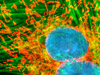
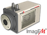 Electron Multiplying Charge-Coupled Devices (EMCCDs)
By incorporating on-chip multiplication gain, the electron multiplying CCD achieves, in an all solid-state sensor, the single-photon detection sensitivity typical of intensified or electron-bombarded CCDs at much lower cost and without compromising the quantum efficiency and resolution characteristics of the conventional CCD structure.
Product Information

Interactive Flash Tutorials
Convolution Kernel Mask Operation
A powerful array of image-processing technologies utilize multipixel operations with convolution kernel masks, in which each output pixel is altered by contributions from a number of adjoining input pixels. These types of operations are commonly referred to as convolution or spatial convolution. This interactive tutorial explores how a convolution operation is performed on a digital image.
The tutorial initializes with an ensemble of random pixel brightness values appearing in the Input Image window. The numerical brightness value of each pixel in the Input Image is displayed in the Digital Image with Kernel Overlay window. In the latter window, the currently selected kernel mask (indicated in red) is superimposed over an ensemble of pixels, where the central pixel lying under the convolution mask is highlighted in blue. The Output Image window displays the pixels that result from the convolution operation. Those pixels lying along the border of the Output Image window are not altered by the convolution operation, but are copied directly from the input image pixel ensemble. The pixels displayed in the Output Image window that result from the convolution operation are distinguished by a slight reddish coloration. To operate the tutorial, select a convolution kernel from the Choose A Kernel pull-down menu, and use the Manual or Auto buttons to advance the tutorial to the next step in the convolution process. When the Auto button is selected, the Auto Speed slider sets the rate at which the tutorial advances to the next step of the convolution operation. Clicking the Reset button will randomize the input pixel ensemble and will allow the user to restart the convolution operation.
In the simplest form, a two-dimensional convolution operation on a digital image utilizes a box convolution kernel. Convolution kernels typically feature an odd number of rows and columns in the form of a square, with a 3 x 3 pixel mask (convolution kernel) being the most common form, but 5 x 5 and 7 x 7 kernels are also frequently employed. The convolution operation is performed individually on each pixel of the original input image, and involves three sequential operations, which are presented in Figure 1. The operation begins when the convolution kernel is overlaid on the original image in such a manner that the center pixel of the mask is matched with the single pixel location to be convolved from the input image. This pixel is referred to as the target pixel (monitor the Position Kernel Mask step in the tutorial).
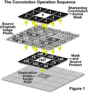
Next, each pixel integer value in the original (often termed the source) image is multiplied by the corresponding value in the overlying mask (the Multiply Kernel with Image step in the tutorial). In the third step, the sum of products from the second step is computed (the Sum Products step in the tutorial). Finally, the gray level value of the target pixel is replaced by the sum of all the products determined in the third step (the Store Output Value step in the tutorial). To perform a convolution on an entire image, this operation must be repeated for each pixel in the original image. Typically, the output gray level value is scaled to match the storage range, although this step is not illustrated in the tutorial.
In general, the numerical values utilized in convolution kernels tend to be integers with a divisor that can vary depending upon the desired operation. Also, because many convolution operations result in negative values (note that the value of a convolution kernel integer can be negative), offset values are often applied to restore a positive value. The smoothing convolution kernel included in the tutorial has a value of unity for each cell in the matrix, with a divisor value of 9 and an offset of zero. Kernel matrices for 8-bit grayscale images are often constrained with divisors and offsets that are chosen so that all processed values following the convolution fall between 0 and 255. Many of the popular software packages have user-specified convolution kernels designed to fine-tune the type of information that is extracted for a particular application.
Convolution kernels are useful for a wide variety of digital image processing operations, including smoothing of noisy images (spatial averaging) and sharpening images by edge enhancement utilizing Laplacian, sharpening, or gradient filters (in the form of a convolution kernel). In addition to convolution operations, local contrast can be adjusted through the application of maximum, minimum, or median filters that rank the pixels within each local neighborhood. Furthermore, the use of a Fourier transform to convert images from the spatial to the frequency domain makes possible another class of filtering operations. The total number of algorithms developed for image processing is enormous, but several operations enjoy widespread application among many of the popular image processing software packages.
Contributing Authors
Kenneth R. Spring - Scientific Consultant, Lusby, Maryland, 20657.
John C. Russ - Materials Science and Engineering Department, North Carolina State University, Raleigh, North Carolina, 27695.
Christopher Steenerson and Michael W. Davidson - National High Magnetic Field Laboratory, 1800 East Paul Dirac Dr., The Florida State University, Tallahassee, Florida, 32310.